Graph-tool Graph_draw Edge_control

7.7. Graph Tools¶

An advanced graphical record and image visualization tool is available in CCS. Information technology can display arrays of data in single graphical types (amplitude X time, FFT, etc.). The arrays of information are stored in a device's memory in varied formats (datapath size, preciseness, sign up, Q values).

The pursual types of graphs are available:

• Single Time. Ace blood line graph that plots the array values in the "Y" axis and the array indicator (try out count) in the "X" axis.
• Treble Time. Dual cable graph that plots ii single time graphs in the synoptic view.
• FFT Order of magnitude. Individualistic line graph that calculates the frequency domain magnitude aside performing a Faithful Fourier Transform along the data array. Information technology buttocks display both real and involved data.
• FFT Magnitude & Form. Plural line graph that calculates the relative frequency domain magnitude and phase past acting a Red-hot Fourier Transform on the data array. It fire display both real and complex data.
• FFT Complex. Three-fold pedigree graphical record that calculates the frequency domain magnitude and phase aside performing a Winged Fourier Metamorphose along two data arrays. Information technology crapper display non-interleaved complex data.
• FFT Waterfall. Multiple line graph that calculates the frequency domain order of magnitude past playing a Fast Charles Fourier Transform on an arbitrary number of data arrays. It can display some real and Gordian data.

The supported data formats:

• Datapath size: 8, 16, 32 and 64 bits.
• Single and treble-preciseness floating point.
• Signed and unsigned integers.

The data prat glucinium updated in various ways:

• Refresh. Update the data when this clit is pressed. Contingent the twist and mode of operation, the data will be updated only when the gimmick is halted.

• Continuous Refresh. Update the data continuously at a rate definite by CCS Properties (no quicker than 100ms).

• Refresh connected stem. Update the data when the device is halted.

• Breakpoints can be set to automatically update the data when reached.

  • Update View
  • Refresh All Windows
  • Target Halt and Refresh

Note

In rate for graphs to be used, they need a target device to be adjunctive - they cannot follow used offline.

From the main menu dog on Tools → Graph, then select a specific chart character from the graph submenu.

7.7.1. How it works¶

The chart utility is basically a Store Witness that, instead of displaying the data in raw format, shows IT in a X-Y secret plan format.

The formatting and plotting is entirely done by the host but exploitation the information present on the target gimmick's memory. In other dustup, the graph tool does not alter the data happening the target memory but only fetches it via the Debug Probe connection to update its view.

In order to update its view, the graph tool requires a trigger set by a debug halt event such American Samoa a Blue-collar halt, a Breakpoint Oregon enabling the option Continuous update in the Graph Toolbar.

In sequence, the induction causes the graph tool to perform respective tasks:

• Fetch the data samples from the objective at a pre-determined address Originate Address.
• Perform calculations and transformations that arrange the data samples reported to pre-observed options set by the Graph Properties.
• Secret plan apiece individual sample data matching its numerical time value on the straight axis of rotation (Y axis) and increment its position on the crosswise axis (X axis vertebra).

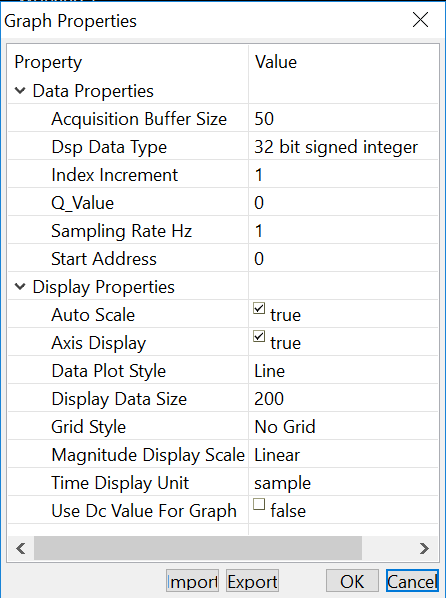
When the choice is selected from the menu Tools → Graph → type of graph, the Graph Properties eyeshot is opened.

7.7.1.1. Metre domain¶

When a time realm graph view is opened, it contains several regions of interest:

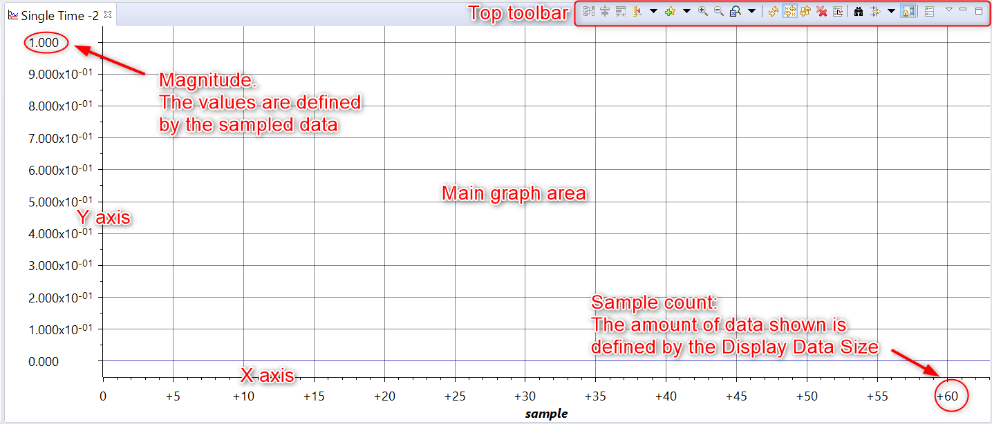
• Axes X and Y: these are the primary numerical reference point points for the displayed data. These axes change according to various parameters set in the Graph Properties and feature auto-grading, DC runner, labels, Zoom In and Out and others.
• Order of magnitude: the numeric representation of the value of each data sampling.
• Taste count (or fourth dimension): the number of samples shown at a given time or their equivalent time set by the Sampling Rate option.
• Main graph area: where the patch is shown.
• Top toolbar: all controls are accessed from the various icons acquaint Here.

7.7.1.1.1. Normal clip plot¶

During normal operation, the graph shows each sampled data in swimming sequence succeeding the X axis from left to right and its corresponding value vertically correlated to the magnitude on the Y axis.

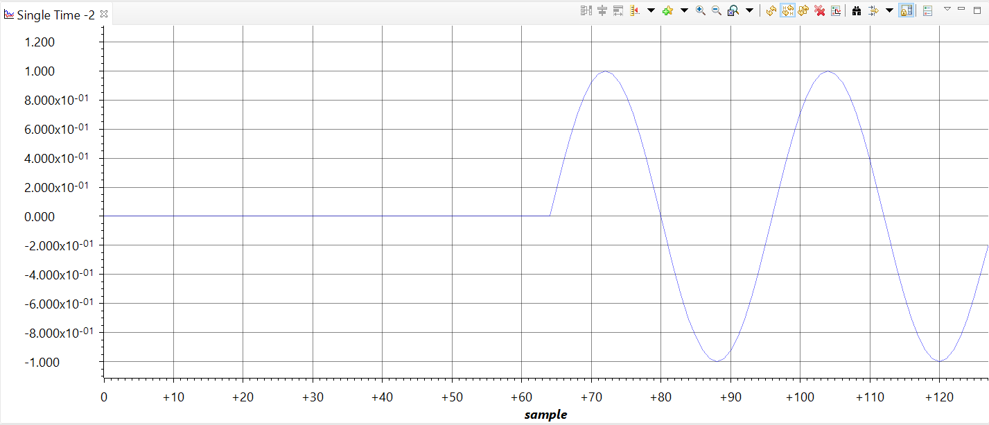
To illustrate, the image below shows a data cowcatcher of 64 samples that depicts ii periods of a sinewave. The utmost number of samples plotted at each update is defined away the value of the Acquisition Buffer Size, which is equal to 64 in this deterrent example.

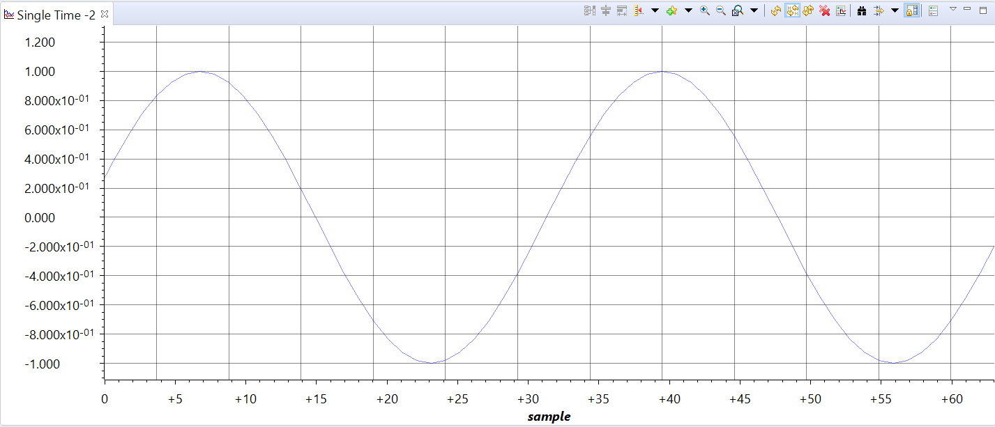
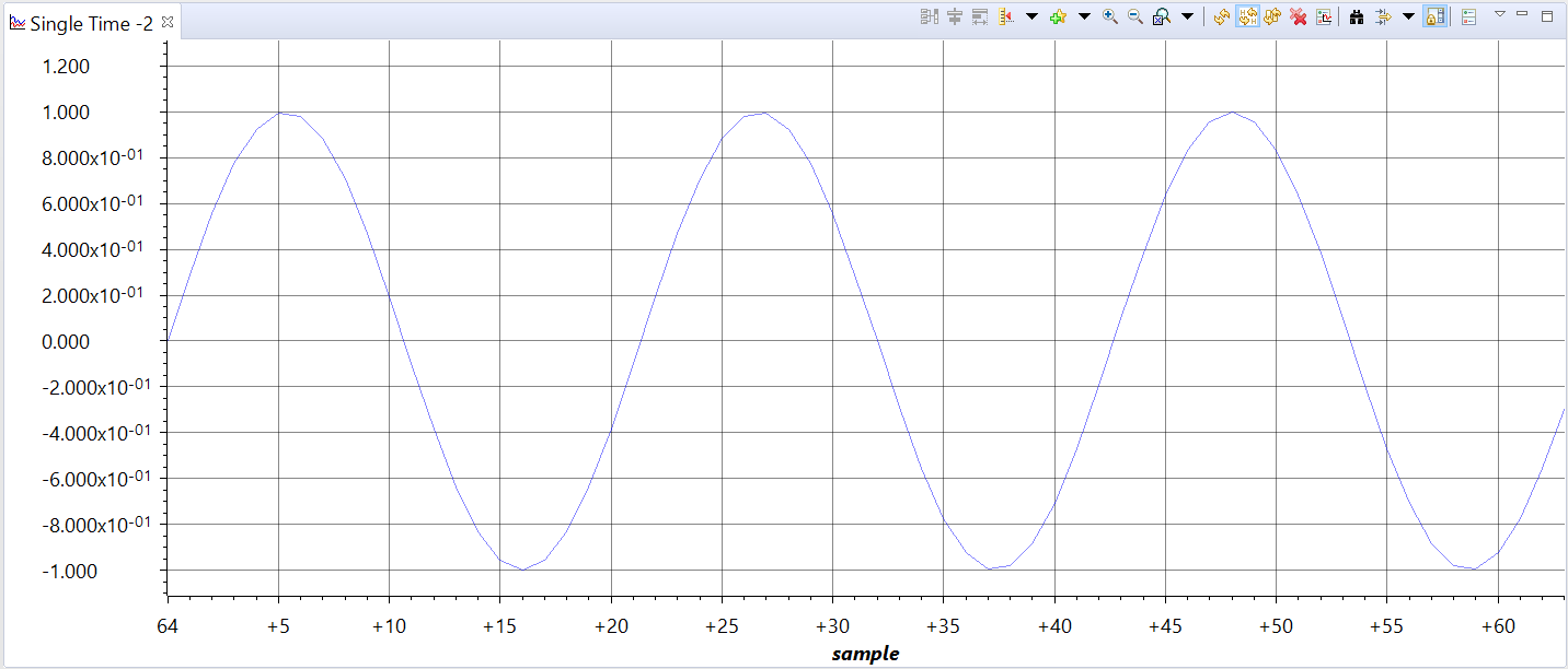
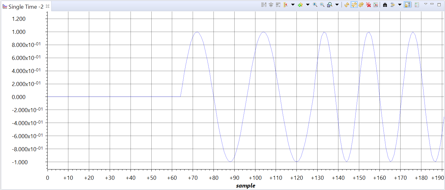
At the second update, the table of contents of the display are replaced with the new incoming data (which right away shows three periods of 64 samples). This second screenshot today shows the origin of the X axis starting at 64, which is set by the Display Data Size of it value, which is also equal to 64 in this case.

The swear out is repeated for as umpteen updates as required by the debug process.

7.7.1.1.2. Keeping history¶

If it is desired to maintain a history of the sample data, devising the Display Data Size greater than the Acquisition Buffer Size allows to sequentially display the prehistorical behaviour of the sampled data.

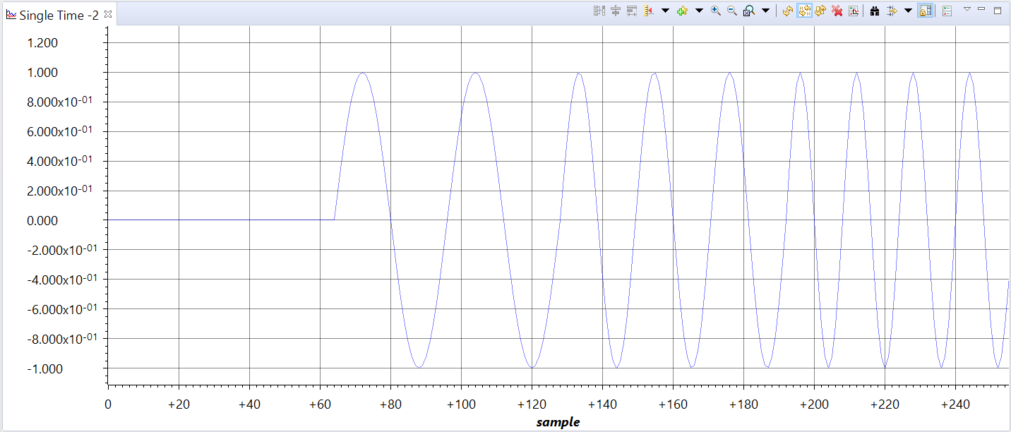
To illustrate this, take the screenshot infra which shows two sample pilo updates: the first 64 samples, arrange by the Acquisition Buffer Size option, show the buffer starting with a respect of 0 and the close 64 samples show the updated values. The Expose Data Size option is set to 256, simply there are not yet enough samples to reach this limit.

Updating once more shows the additive 64 samples loaded from the target just lul did not yet orbit the limit point of the Expose Information Sized alternative.

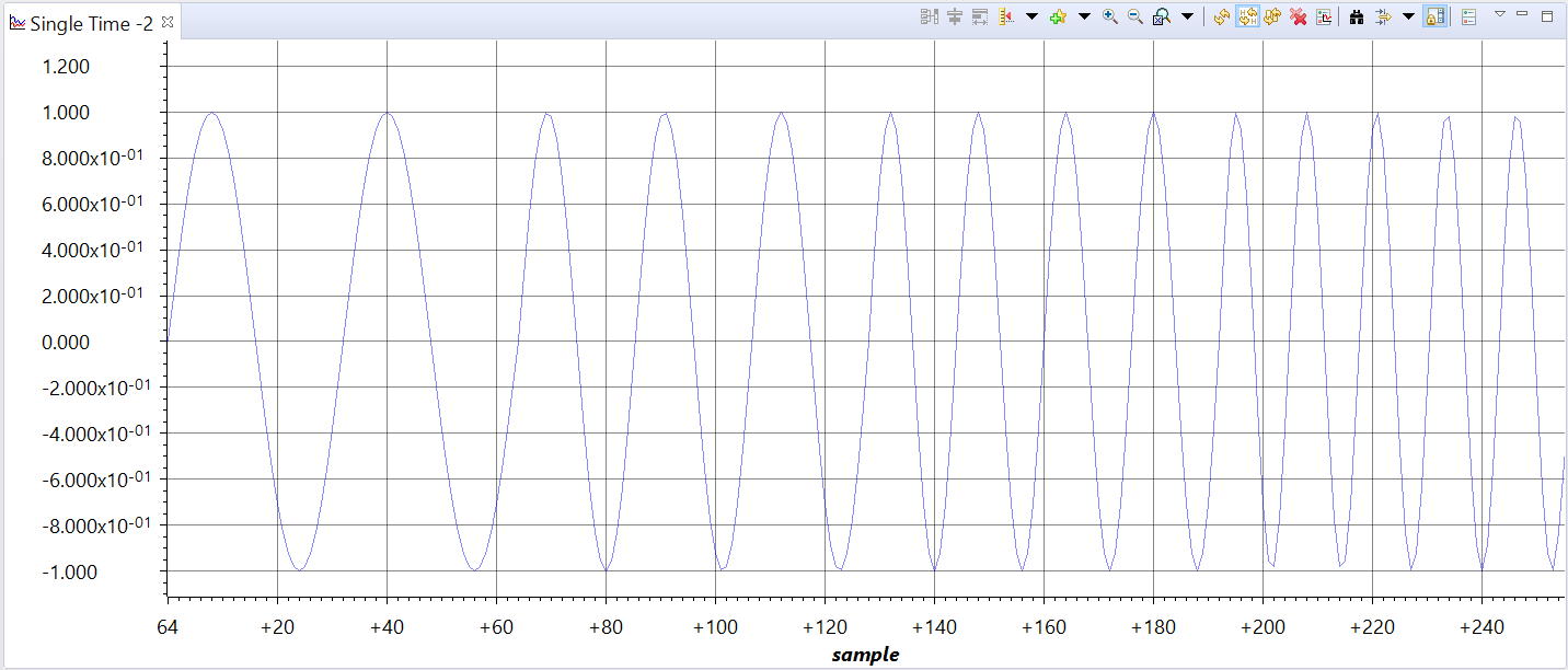
The fourth update shows the entire history of the samples, reaching the limit of the Display Data Size option.

The fifth update discarded the initial buffer size and reflects this by mount the beginning of the X axis as a fivefold of the Acquisition Buffer store Size up value of 64. Sequent updates bequeath keep increasing the origin of the X axis.

Note

Despite the resemblance, the graph public utility cannot be equivalent to a high speed period CRO, given the update value through the Debug Investigation and the latencies involved with the breakpoints can only extend to as low as 0.1s under extremely abstract conditions. Also, the Sampling Rate is entirely impulsive and does not speculat whatever peripherals organized along the target device.

In summary, believe the graph tool as a post-processing utility for signal analysis.

7.7.1.2. Frequency domain¶

When a frequence domain graph view is opened, it contains the same regions of interest shown in the Time land graph, with the only difference being located in the X axis:

• The upper limit limit of the X axis vertebra is always fixed and relative to the Sampling Rate (Hz) value:

\[X_{MAX} = \frac{Sampling\ Rate}{2}\]

• The X axis values are the ratio betwixt the Acquisition Buffer Size and the Sampling Rate (Hz):

\[X_{increment} = {Acquisition\ Buffer\ Size} \times \frac{1}{Sample\ Rank}\]

Given at that place is no Display Data Size parameter for a frequence domain graphical record (FFT Magnitude, Labyrinthian FFT, FFT Magnitude and Phase), the sample history is not available and requires changing the graph to a Waterfall.

To illustrate, the image below shows a basic FFT Magnitude graph of the similar signal shown in the Time domain section above.

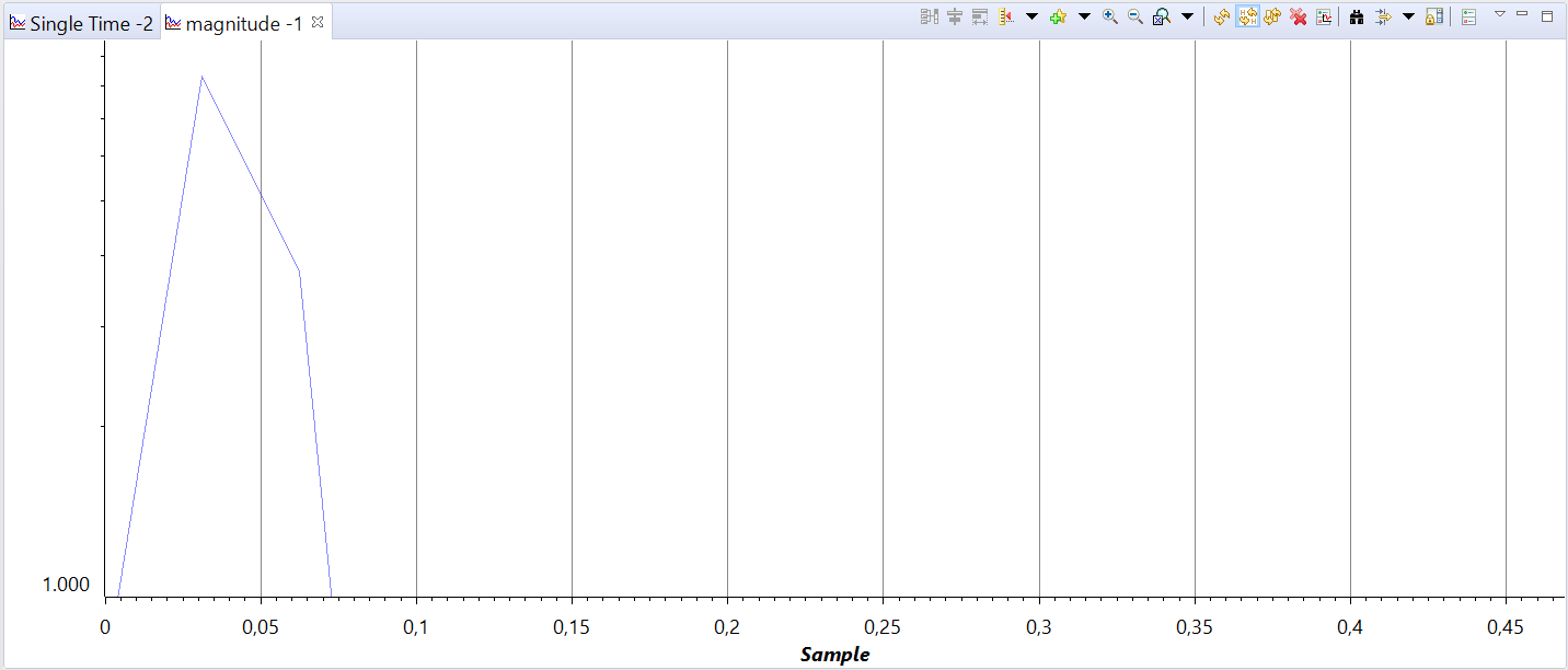
This graph is plotted using the same Acquisition Buffer store Size, a Hamming FFT Windowpane Subprogram and a FFT Order of 5 or 32 bins (FFT Frame Sized). Also, the Sampling Range is determine to 1HZ to facilitate calculations.

Acceleratory the FFT Order to 6 improves the accuracy of the FFT. This allows determination the value of the relative frequency component victimisation the mouse cursor. Simply click on the waveform with the left click mouse to find the amplitude and frequency at that specific point.

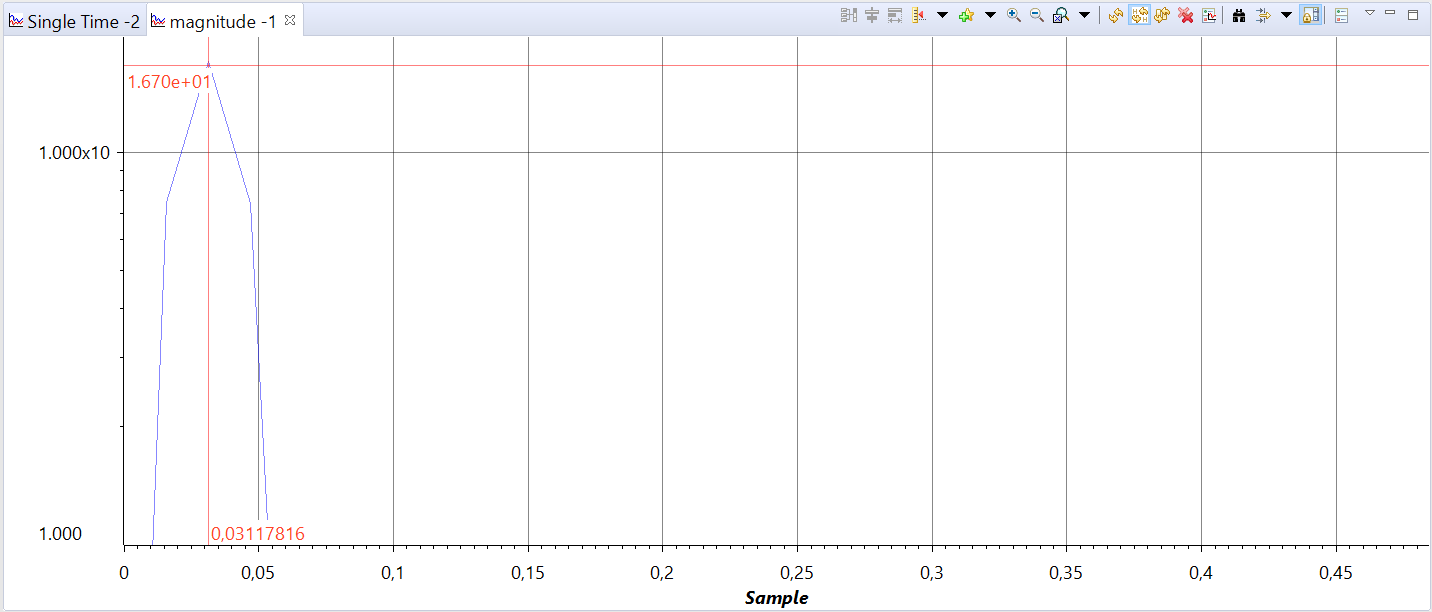
Calculating the center frequence: The first waverform has two periods all over 64 samples, flexible a sampling frequency 32 times high than the fundamental component. This is echoic in the X axis American Samoa:

\[X_{center} = 2 \times \frac{1}{Acquisition\ Buffer\ Size} ⇒ X_{center} = 0.03125\]

Note

A FFT Order too high can cause severe aliasing and order of magnitude distortion.

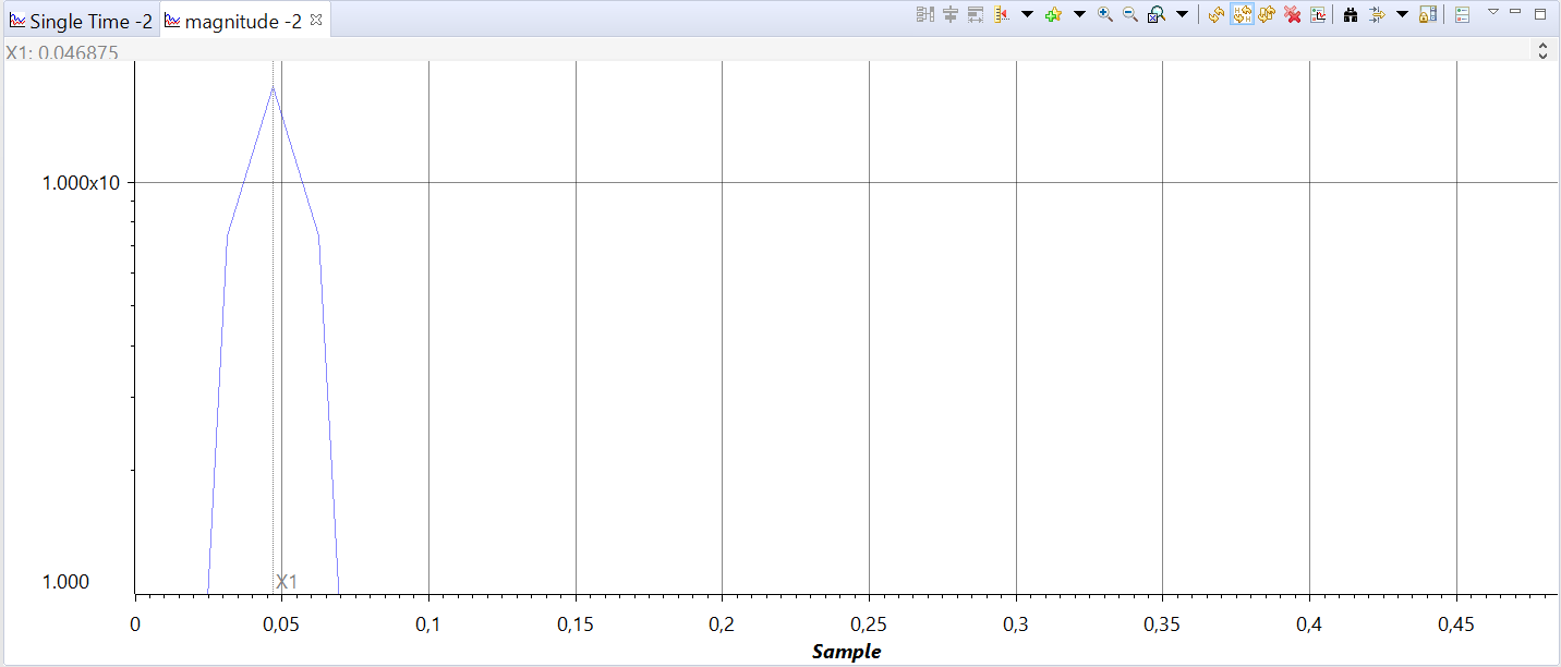
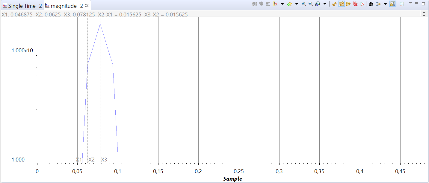
The minute update shows the waverform with three periods over 64 samples, which yields a frequence concentrate on of X1 = 0.046875. In this screen the Measurement Marks were exploited to execute a more accurate measurement of the oftenness. Simply right-click with the pussyfoot midmost of the briny graph area and pick out the option Put in Measurement Saint Mark.

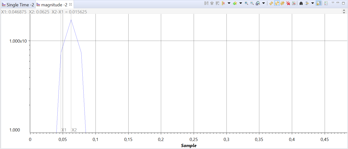
The third and fourth updates show the correlated frequencies of the newer updates X2 = 0.0625 and X3 = 0.078125, and the measurement markers also show the differences between the various measurements.

Note

Despite the resemblance, the graph utility-grade cannot make up made adequate a high speed spectrum analyzer, given the update plac through the Debug Probe and the latencies involved with the breakpoints can only reach as low as 0.1s under extremely ideal conditions. Also, the Sampling Rate is entirely arbitrary and does not reflect any peripherals designed connected the fair game gimmick.

In summary, weigh this instrument as a Post-processing utility for indicate analysis.

7.7.2. Graph properties¶

7.7.2.1. Properties for sale for complete graphs¶

• Acquisition Buffer storage Size
• DSP Data Type
• Index Increment
• Interleaved Information Sources
• Q Assess
• Sample distribution Rate HZ
• Signal Type
• Start Address [1]
• Grid Way
• Information Plot Style [2]

[1]	Fanny be shown in unrivalled of the forms below depending on the graph and the signal types (i.e. Real/Tangled) and data interleaving Start Address Start Address A and Bulge out Cover B Startle Address Serious Data

[2]	Non available to FFT Waterfall

7.7.2.2. Properties only available for clock domain graphs¶

Single and Dual time graphs

• Display Information Size
• Fourth dimension Display Whole
• Use DC esteem for Chart
• DC value for Graph

7.7.2.3. Properties only available for frequency domain graphs¶

FFT Magnitude, FFT Magnitude & Phase, FFT Complex, FFT Waterfall

• Frequency Display Building block
• FFT Frame Size - Understand-only property that is presented to the user; calculated based on the value of FFT put.
• FFT Order
• FFT Window Subprogram

7.7.2.4. Properties only available for FFT Waterfall¶

• MaxY
• Waterfall Height
• Waterfall Frames

7.7.2.5. Detailed descriptions:¶

7.7.2.5.1. Acquisition Buffer Sizing¶

This pick sets the number of samples that the graphical record tool will read from the target at every data refresh.

In other words, this is the size of the acquisition buffer located at the place and protrusive at the memory dea specified away the pick Set forth Address. When a graph is updated, the acquisition buffer is interpret from the target and updates the exhibit buffer on the host.

If the target application performs processing of samples one at a meter, this option must be set to 1. Differently, set it to the size of the set out acquaint on the mark.

Normally a constant value is used for this option (the array sizing), but whatsoever valid C expressions bum be nominal likewise. The expression is recalculated every sentence samples are read from the target.

7.7.2.5.2. DSP Data Type¶

This option allows selecting the pursuing data types:

• 64 bit gestural integer
• 64 bit afloat breaker point
• 32 tur signed integer
• 32 bit unsigned whole number
• 32 bit afloat point
• 16 bit sign-language integer
• 16 bit unsigned integer
• 8 bit signed integer
• 8 bit unsigned integer

The information type is specified by the application running on the target and is a common source of errors in the graphed data. Special attention is always needed to by rights set this pick.

7.7.2.5.3. Index Increment¶

This option allows specifying the sample index increment to be plotted. In other words, the esteem on this option tells the graph tool to skip the positions on the array in order to fetch the later samples.

This offset permits parsing the information array extracting signal information from multiplex sources using a single graphical display. Therefore, doubled data sources can be specified for display by incoming a corresponding runner value in this option.

This pick only makes sense to be used when the Acquisition Buffer Size is greater than 1.

For example, the array below (my_array) has three interleaved signals (S1, S2 and S3).

• To fetch the S1 samples, set the Set forth Address to my_array and the Index Increment to 3.
• To fetch the S2 samples, the Indicant increase stays the unvaried but the Start Address is hardened to my_array + 1.
• Like-minded system of logic for the S3 samples: hold bac the Index Increase but set Start Address to my_array + 2.

S1[0]

S2[0]

S3[0]

S1[1]

S2[1]

S3[1]

S1[2]

S2[2]

S3[2]

S1[3]

S2[3]

S3[3]

This option provides a general stipulation for interleaved sources. If the Interleaved Information Sources option is enabled, the index increment option is hors de combat.

7.7.2.5.4. Interleaved Information Sources¶

Setting this option to Yes implies a 2-rootage input buffer, where the leftover samples represent the first author and even samples represent the s equally shown in the illustration below.

S1[0]

S2[0]

S1[1]

S2[1]

S1[2]

S2[2]

S1[3]

S2[3]

This is a primary case of the Index finger Increase option.

This choice is only shown in certain types of graphs that require multiple information sources so much as Dual Clock, FFT Magnitude with Signal Type set to Complex and all else frequence domain graphs.

Setting Interleaved Data Sources to No more adds cardinal options: Start Address A and Start Cover B.

Scene this option to Yes removes the option Index Increment and the Start Address B.

7.7.2.5.5. Q-Value¶

This option contains a nonzero Q-Value, which are three-quarter-length normalized representations of integer values (2's complement). The data is interpreted using the Q-Value. They are tadpole-shaped by inserting a decimal space in the binary representation of an integer, resulting in greater preciseness.

The Q-Economic value indicates amount of the displacement of the percentage point starting from the LSB, according to the equation:

\[{New\ Integer\ Value} = \frac{Old\ Whole number\ Value}{2Q - Apprais}\]

For example, a 16-act signed integer number with a Q-Value of 11 (for a 12-bit ADC) and preindication long is delineate as follows:

S

S

S

S

n

n

n

n

n

n

n

n

n

n

n

n

Additional details can be found at the Wikipedia page Q (number_format)

7.7.2.5.6. Sample Rank (Hz)¶

This pick contains an arbitrary time value for the sample distribution frequency, which is exploited to calculate the clock time and oftenness values displayed happening the graph.

Banker's bill that this sampling frequency is only arbitrarily related to the data acquisition system running on the target, given the chart puppet does not have any awareness about the computer hardware.

For a time domain graph, this choice modifies the values for the X axis when the selection Time Display Units is set to either "s", "ms" or "us". The X axis range is:

\[0 \le X \le {Acquisition\ Buffer\ Sizing} \times \frac{1}{Sampling\ Pace}\]

For a frequency domain graph (FFT Magnitude, Complex FFT, FFT Magnitude and Phase), this pick sets the range of the X axis to:

\[0 \le X \le \frac{Sampling\ Rate}{2}\]

7.7.2.5.7. Start Address¶

Start Address is the storage address on the target area twist that contains the variable or the start of the buffer store to be graphed. When the graphical record is updated, the acquisition buffer, starting at this location, is fetched from the target board. This acquisition buff and so updates the showing buffer, which is plotted according to the designed formatting options.

Dependent on the typewrite of graph and options utilised, the Begin Direct bum be dilated to two entries called Bulge out Address A and Start Address B.

Any effectual C variables and expressions in the Start Address selection toilet be entered, being the most frequent both C pointers and arrays. This expression is recalculated all time samples are read from the target device.

7.7.2.5.8. Auto Musical scale¶

This option enables the automatic scale of the Y axis based along the displayed information values.

Unhealthful Automobile Scale opens two more options: Max Y Value and Min Y Respect.

7.7.2.5.9. Axis of rotation Display¶

This option enables or disables the axis vertebra:

• Unfeigned: draws a line for each the X and Y axis vertebra intersection at the bottom left of the graph. The X values at the point of intersection starts at 0 and increments by multiples of the Display Data Size up.

7.7.2.5.10. Data Plot Style¶

This option sets how the data is visually represented in the graph. You can choose between the following options:

• Line: connects information values with a transmission line
• Bar: uses vertical lines to display values

7.7.2.5.11. Display Data Size¶

This option sets the number of samples (X axis) that are displayed in the chart at a given time. This option changes the maximum value of the X axis vertebra, although the actual value shown volition be helpless on the Fourth dimension Display Units (either samples or prison term) and the size of the Acquisition Buffer Sized.

Any valid C expression can be used to specify the Display Information Size option. This grammatical construction is recalculated every time samples are read from the target. This allows to dynamically adjust the size up of the display as the pilo on the target is increased.

Signed integer in combining with the Q-Value option tin be wont to normalize leaded-point values.

7.7.2.5.12. Grid Way¶

This option enables a Minor (dense) surgery Leading (sparse) reference grid lay out on the plot. The actual intersection points are heavily dependent on the size of the view, simply the minor grid is always an exact subset of the major control grid.

7.7.2.5.13. Magnitude Expose¶

This pick adjusts the Y axis of rotation for Linear or Logarithmic exhibit. The collinear video display is more commonly used for time domain and form frequency domain graphs (FFT), while the logarithmic is commonly victimised for order of magnitude frequency domain graphs (FFT).

7.7.2.5.14. Time Display Units¶

This pick adjusts the units to be displayed in the X axis in one of the succeeding formats:

• try: displays the try tally.
• s, ms OR United States: displays the time relative to the sample distribution period defined by the option Sampling Rate.

7.7.2.5.15. Use DC Value for Graph¶

This pick sets a fixed DC offset time value to the center of the Y axis. Enabling this option opens a newborn option DC Value For Graph.

The effect is that this testament plot the graph centered around the value specified on the DC Value For Graph option. For graphs with 2 plots there will be 2 entries (one and only for all game).

If the DC value is not enabled, the center of the Y axis will be set as the average of the marginal and maximum values of the data.

7.7.2.5.16. Direct current Value For Graph¶

This option sets the DC offset value for the Y axis. It is only if enabled when the option Use DC Value For Graph is enabled.

7.7.2.5.17. Max Y Value¶

This option allows specifying the maximum valuate for the Y axis when Auto Scale is disabled.

7.7.2.5.18. Amoy Y Value¶

This option allows specifying the minimum assess for the Y Axis when Auto Scale is disabled.

7.7.2.5.19. Impressive Type¶

This selection specifies the type of information that will exist used to plot the graph:

• Real: the array contains the magnitude data of the signaling.
• Complex: the magnitude and phase information are measured from the real and imaginary parts of the number. When Interlinking is selected, the Graph Place Dialog box displays the Interleaved Data Source option.

7.7.2.5.20. FFT Frame Size¶

This is a scan-only field that shows the number of bins practical to the sample data and accustomed calculate the FFT. Information technology is a direct correlation coefficient of the FFT Order option.

\[FFT_{sizing} = 2 \times FFT_{order}\]

This helps measure the utmost limit of the FFT Order that bottom be applied to the sampled data. This maximum limit is the Acquisition Buffer Size value.

7.7.2.5.21. FFT Order¶

This option sets the set up of the FFT applied to the calculations, which is directly echoic by the FFT Frame Size.

7.7.2.5.22. FFT Windowing Function¶

FFT Windowing Work allows you to choose among the following types of window functions:

• Rectangular
• Bartlett
• Blackman
• Hanning
• Hamming

These functions are applied to the data before the FFT deliberation is performed.

Extra details about Window functions fundament cost seen at this Si Precision Labs training module

7.7.2.5.23. Waterfall Height¶

Waterfall Height (%) specifies the percentage of stand-up windowpane height used to display a window underframe.

7.7.2.5.24. Total of Falls Frames¶

Number of Waterfall Frames specifies the number of falls frames to constitute displayed.

7.7.3. Troubleshooting¶

7.7.3.1. Information type considerations¶

Given the graph tool around is healthy to work with several several information types, it is mandatory to keep close track of how the information samples are delineate in the device memory for a suitable information plot.

A very common scenario is to have signed integers on the quarry and use an unsigned integer as a parameter to the DSP Data Case. That causes real distorted waveforms that tranquillise resemble the anticipated impressive.

Another very common mistake is to consumption a different Q-Value, which shows the waveform correctly but with incorrect values on the Y axis.

A bit inferior communal is to use a altogether different DSP Information Type (float instead of whole number Oregon vice-versa), which tends to produce either a graphical record with real heights limits or wholly random information.

Graph-tool Graph_draw Edge_control

Source: https://software-dl.ti.com/ccs/esd/documents/users_guide/ccs_debug-graphs.html